Project 05 · Case study
Numerical transport
Maze Concentration Diffusion
A cell-centred finite-volume model that uses transient dye diffusion to reveal the connected route through a maze.
Project overview
Dye transport became a numerical path finder
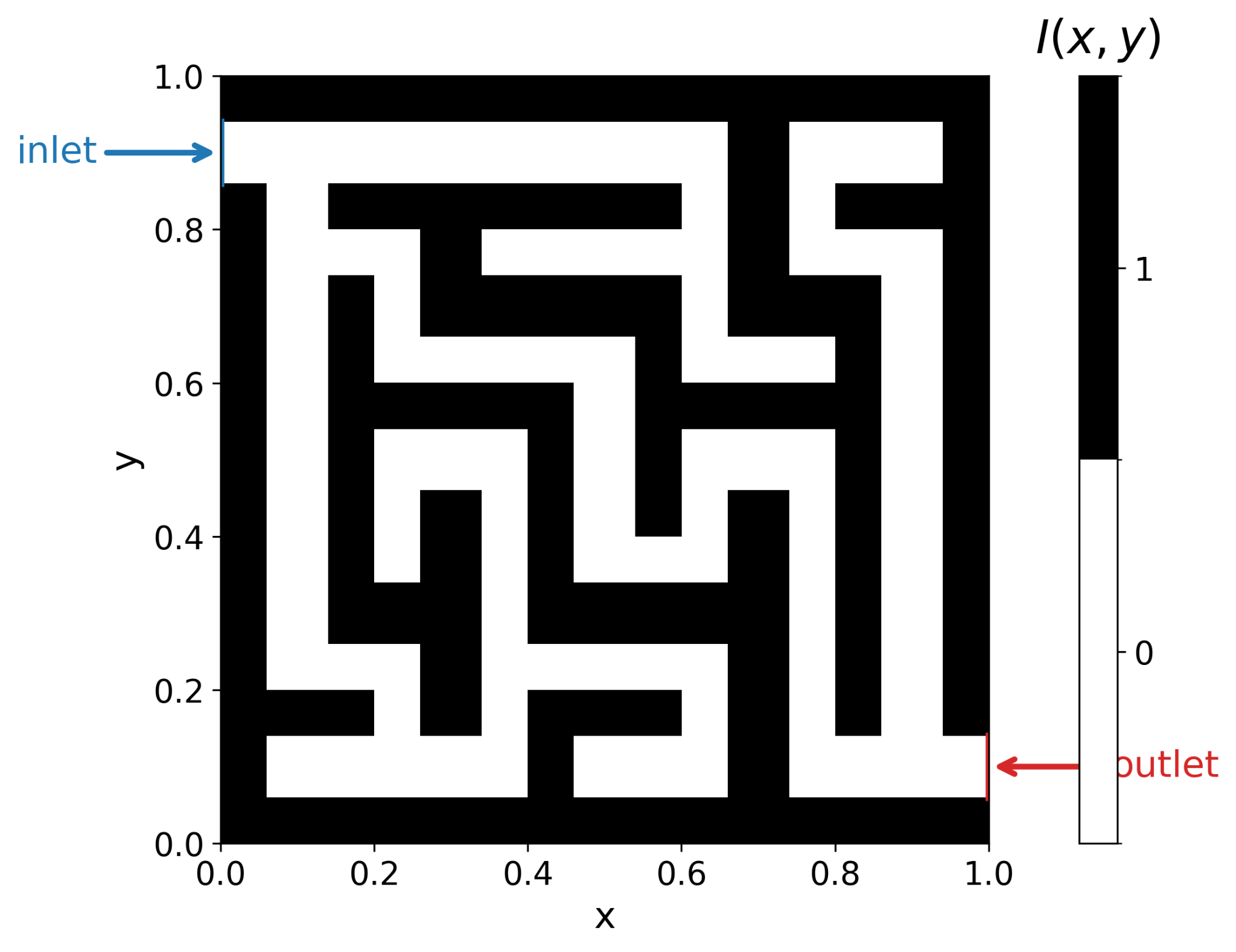
The maze starts with clean water. A fixed dye concentration enters at the upper-left opening while clean water is maintained at the lower-right outlet.
Physical idea
Concentration spreads through connected liquid corridors because the maze walls are assigned a much smaller diffusion coefficient.
Boundary conditions
The inlet and outlet use fixed concentration values. Every other external boundary is treated as no-flux.
Numerical objective
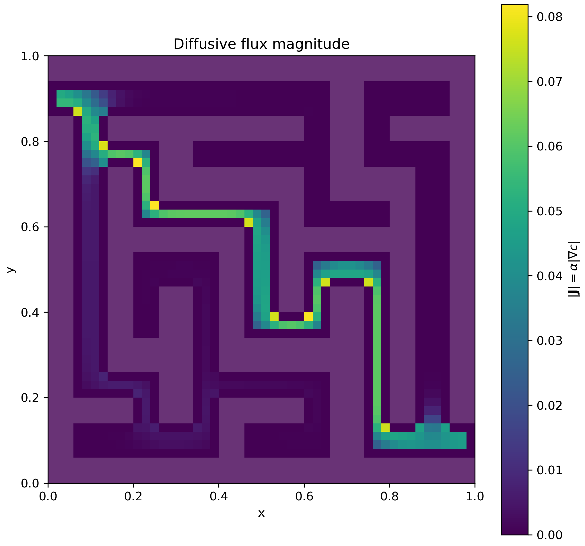
The transient field shows reachability while the near-steady flux magnitude isolates the preferred route through the maze.
Geometry and boundaries
A binary maze became a variable medium
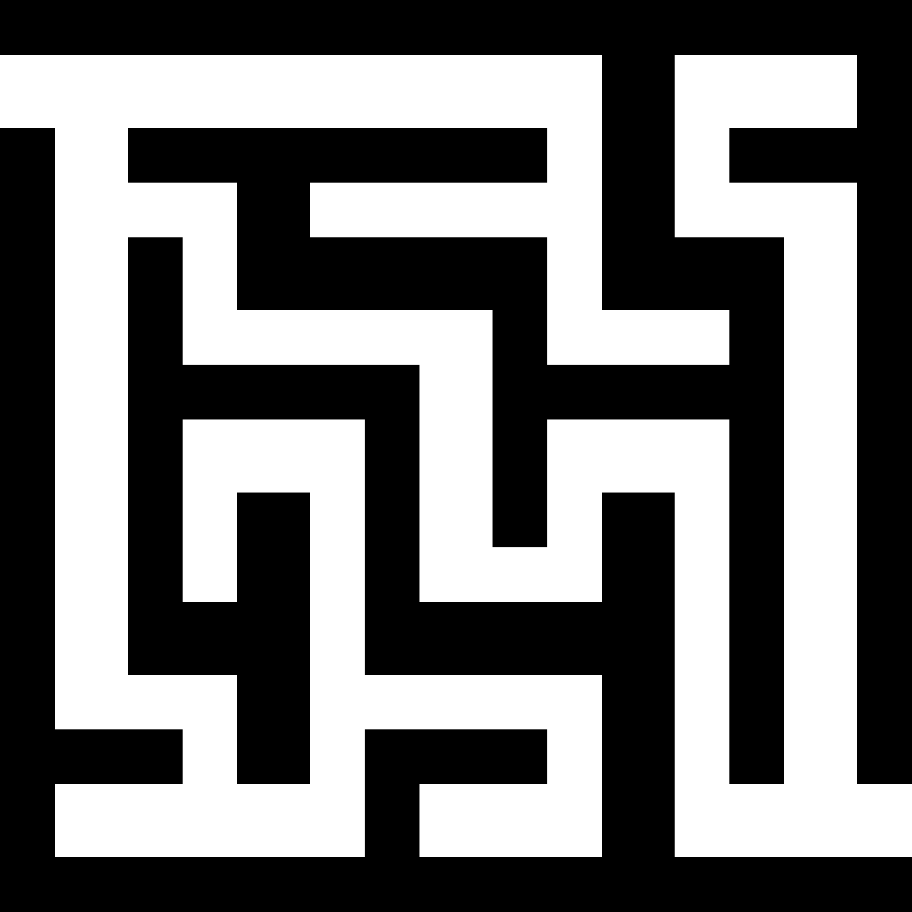
White cells represent water-filled corridors. Black cells represent walls with a diffusion coefficient many orders of magnitude lower.
Numerical model
Flux continuity at every liquid-wall interface
The discontinuous diffusion coefficient makes face treatment the critical modelling detail.
The solver uses a cell-centred finite-volume method. Each control volume balances diffusive fluxes across its faces, ghost cells impose the external boundary conditions and harmonic face interpolation preserves flux continuity at liquid-wall interfaces.
- αliquid
- 10−1
- αwall
- 10−8
- Initial field
- c = 0
- Grid
- 50 × 50
Path extraction
The flux field solved the maze
Near steady state the diffusive flux is approximately continuous along the main inlet-to-outlet path.
Dead ends can contain dye during the transient but they do not sustain a through-flux. Their diagnostic magnitude therefore weakens while the connected path remains visible.
Engineering outcome
A transport equation used as a decision tool
The project connected physical diffusion, discontinuous material properties, boundary-condition treatment and numerical stability in one compact solver.